Study species and sampling design
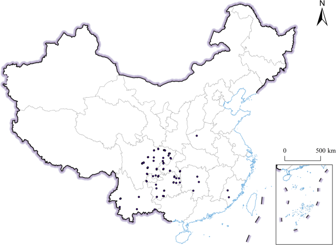
Neosinocalamus affinis is a sympodial, pachymorph bamboo reaching 5–10 m in height, with narrow lanceolate leaves 8–20 cm long and 1–3 cm wide. Leaves of N. affinis were collected from 38 county-level sites distributed across seven provinces in southern China (Chongqing, Fujian, Guizhou, Henan, Hunan, Sichuan and Yunnan) during the 2023 and 2024 growing seasons (May–September; Table 1; Fig. 1). Sites spanned 37–1,854 m in elevation, 9.9–20.6 °C in mean annual temperature (MAT) and 651–1,559 mm in mean annual precipitation (MAP), covering most of the climatic envelope of the species.
At each site, 3–8 mature, healthy bamboo clumps were randomly selected at least 10 m apart to minimise clonal dependence, avoiding edge individuals, recently disturbed stands and clumps showing visible signs of pest damage or nutrient deficiency. From each clump, fully expanded, sun-exposed leaves were sampled from current-year culms (2–3 years old) at mid-canopy height (approximately 2/3 of total height) on south-facing branches to standardise light environment. Only fully expanded, non-senescent leaves from the middle portion of leafy branches were retained. Within each clump, 3–10 leaves were pooled to form a clump-level sample, and 2–8 clump-level samples were averaged to produce the site-level observations analysed here. This procedure yielded 162 site-level observations across the 38 sites. Plant material was formally identified by Miao Liu (co-author) at the International Center for Bamboo and Rattan, Beijing. Voucher specimens were deposited in the herbarium of the Key Laboratory of National Forestry and Grassland Administration for Bamboo & Rattan Science and Technology (herbarium code: ICBR; voucher numbers ICBR-Neosinocalamus-2023001 to 2023038).

Geographic distribution of the 38 county-level sampling sites of N. affinis across seven provinces in southern China. Sites span 37–1,854 m in elevation, 9.9–20.6 °C MAT and 651–1,559 mm MAP.
Morphological measurements
For each leaf, we measured: (i) leaf length (L, cm), from the base of the lamina to the apex along the midrib, with digital calipers (Mitutoyo CD-15CPX, Japan; precision 0.01 mm); (ii) maximum leaf width (W, cm), perpendicular to the midrib, with the same calipers; (iii) leaf thickness (LT, mm), averaged over three non-vein positions in the middle third of the lamina using a digital micrometer (Mitutoyo MDH-25 M, Japan; precision 0.001 mm); and (iv) leaf area (LA, cm²), measured on fresh leaves with a portable leaf-area meter (LI-3000 C, LI-COR Biosciences, Lincoln, NE, USA). The L/W ratio (dimensionless) was calculated as L / W for each leaf and then averaged at the clump and site level.
Biomass and dry-matter traits
After morphological measurements, leaves were weighed for fresh mass (FW, g) using an analytical balance (Sartorius BSA224S, Germany; precision 0.1 mg), then oven-dried at 65 °C for 72 h until constant mass and re-weighed for dry mass (DW, g). SLA (cm² g⁻¹) was computed as LA / DW, and LDMC (%) as (DW / FW) × 100.
Chlorophyll and photosynthetic performance
Leaf chlorophyll content was estimated with a SPAD-502Plus chlorophyll meter (Konica Minolta, Japan); three readings were taken along each leaf and averaged to yield a single SPAD value. Chlorophyll a fluorescence parameters were measured on fully dark-adapted leaves using a portable pulse-amplitude-modulated fluorometer (PAM-2500, Heinz Walz, Germany) after 30 min of dark adaptation with leaf clips. Measured parameters included minimum fluorescence (Fo), maximum fluorescence (Fm), variable fluorescence (Fv = Fm − Fo), maximum photochemical efficiency of PSII (Fv/Fm), photochemical quenching coefficient (qP) and non-photochemical quenching (NPQ). Measurements were taken on cloud-free mornings between 08:00 and 11:00 local time.
Leaf carbon, nitrogen and phosphorus
Dried leaves were ground to a fine powder using a ball mill (Retsch MM400, Germany) and passed through a 0.15 mm sieve. Total leaf carbon (TC, g kg⁻¹) and total leaf nitrogen (TN, g kg⁻¹) concentrations were determined by dry combustion on an elemental analyser (Vario MACRO cube, Elementar Analysensysteme GmbH, Langenselbold, Germany) using approximately 40 mg of leaf powder per sample. For leaf phosphorus (TP, g kg⁻¹), approximately 100 mg of ground sample was digested in a mixture of concentrated H₂SO₄ and H₂O₂, and P concentration in the digest was determined colorimetrically using the molybdenum-antimony-ascorbic acid method on an ultraviolet–visible spectrophotometer (UV-2600, Shimadzu, Japan) at 700 nm. Stoichiometric ratios C: N, N: P and C: P were calculated on a mass basis.
Environmental variables
Geographic coordinates (longitude, latitude) and elevation were recorded in the field with a handheld GPS unit (Garmin GPSMAP 64s, USA; precision ± 3 m). Mean annual temperature (MAT, °C), mean annual precipitation (MAP, mm), maximum temperature of the warmest month and minimum temperature of the coldest month were extracted for each sampling coordinate from the WorldClim 2.1 global climate database at 30-arc-second (~ 1 km) resolution40, representing long-term climatic conditions averaged over 1970–2000. At each clump, topsoil samples (0–20 cm) were collected after removing the litter layer; soil water content (SWC, %) was determined gravimetrically after drying at 105 °C for 24 h, and soil bulk density (SBD, g cm⁻³) was measured using the cutting-ring method (volume 100 cm³). All environmental variables were assigned to site-level observations by averaging over clumps at each site.
Statistical analysis
All analyses were conducted in Python 3.10 using NumPy, SciPy, pandas, scikit-learn, statsmodels and matplotlib. The significance threshold was α = 0.05. Variables were inspected for normality (Shapiro–Wilk test) and homogeneity of variance (Levene test) before parametric procedures.
To define L/W-based shape classes in a data-driven way, we applied k-means clustering to the L/W ratio of all 162 site-level observations for k = 2 to k = 6, with 10 random initialisations and a fixed random seed. The optimal k was selected using the silhouette coefficient, complemented by visual inspection of the L/W frequency distribution to ensure that the resulting classes were biologically interpretable. The resulting cluster boundaries are reported in the Results.
For leaf-area estimation we compared four candidate models on the complete site-level dataset: (i) a pooled Montgomery equation, LA = k · L · W, with a single proportionality coefficient fitted by least squares through the origin; (ii) a pooled multiple linear regression, LA = a + b₁L + b₂W; (iii) a class-specific Montgomery model with a separate k for each shape class; and (iv) a class-specific MLR with separate intercept and slope coefficients for each shape class. Including the class-specific Montgomery model alongside the pooled MLR allows us to disentangle the contribution of shape stratification from the contribution of the more flexible MLR functional form. Model performance was compared using the coefficient of determination (R²), root-mean-square error (RMSE) and Akaike information criterion (AIC).
Differences in functional traits among shape classes were tested by one-way ANOVA, and pairwise comparisons were performed using Tukey’s honestly significant difference (HSD) post-hoc test. Pairwise Pearson correlations were computed among all leaf traits. Conclusions focus on correlations that are both statistically significant and of non-trivial magnitude (|r| ≥ 0.30).
To assess the drivers of leaf functional trait variation, we proceeded in two steps. First, we computed pairwise Pearson correlations between each focal leaf trait (LA, L/W, LT, SLA, LDMC, TN, TP, SPAD, Fv/Fm, TC) and each environmental variable (elevation, MAT, MAP, SWC, SBD and latitude). Second, we fitted multiple linear regression models in which each focal trait was regressed on the full set of standardised environmental variables in order to estimate their joint and partial contributions; model fit was summarised by R² and overall F-test p value. Variables were standardised (mean = 0, SD = 1) prior to MLR so that regression coefficients are directly comparable in magnitude.
To assess the relative importance of within-site versus among-site variation, we partitioned the total sum of squares of each focal trait into within-site and among-site components based on a one-way ANOVA framework with site (county) as the grouping factor. The within-site sum of squares was the residual within-group SS, and the among-site sum of squares was the between-group SS; the percentage of total trait variance attributable to within-site variation was computed as 100 × SS_within / (SS_within + SS_among). Because climatic variables are identical for all observations within a given site, the within-site percentage represents an upper bound on the trait variation that is intrinsically unexplainable by among-site climate.